Text Mining in R: Word Count Analysis
We are going to extract wordcounts from texts and visualize the results in R. Firstly, you need to install the tidytext and readtext packages.
# Install packages
install.packages("tidytext")
install.packages("readtext")
install.packages("magrittr")
Installing package into 'C:/Users/elibo/Documents/R/win-library/4.0'
(as 'lib' is unspecified)


package 'tidytext' successfully unpacked and MD5 sums checked

The downloaded binary packages are in
	C:\Users\elibo\AppData\Local\Temp\Rtmp2Fs3XH\downloaded_packages


Installing package into 'C:/Users/elibo/Documents/R/win-library/4.0'
(as 'lib' is unspecified)


package 'readtext' successfully unpacked and MD5 sums checked

The downloaded binary packages are in
	C:\Users\elibo\AppData\Local\Temp\Rtmp2Fs3XH\downloaded_packages


Installing package into 'C:/Users/elibo/Documents/R/win-library/4.0'
(as 'lib' is unspecified)


package 'magrittr' successfully unpacked and MD5 sums checked

The downloaded binary packages are in
	C:\Users\elibo\AppData\Local\Temp\Rtmp2Fs3XH\downloaded_packages
# Load packages
library(tidytext)
library(readtext)
library(magrittr)
I will use Charles Dickens’ Our Mutual Friend for the word count analysis. I downloaded the txt file on Gutenberg (https://www.gutenberg.org/). Now, we need to load the text file into the R program.
Before loading files, we should find the working directory. Let’s find where is the working directory by using the getwd function.
getwd()
‘C:/Users/elibo/Downloads’
Depending on the OS, the format of the file location is different. For Mac OS, the location begins with ~/ whereas in Windows, the location begins with C:\ I have the txt file in ~/desktop/ In the readtext function, you need to put the location of the file.
# Change the URL
omf <- readtext("OMF.txt", encoding="utf-8")
Let’s check the loaded file in R. Type summary() and the file name.
summary(omf)
    doc_id              text
 Length:1           Length:1
 Class :character   Class :character
 Mode  :character   Mode  :character
Tokenize the text file
Now, we need to tokenize the text file. We are going to use “unnest_tokens” included in the Tidytext package (from v.0.2.0). You can find specifics for the usage of the “unnest_tokens” in the following link: (https://www.rdocumentation.org/packages/tidytext/versions/0.2.0/topics/unnest_tokens)
install.packages("tidyr")
Installing package into 'C:/Users/elibo/Documents/R/win-library/4.0'
(as 'lib' is unspecified)


package 'tidyr' successfully unpacked and MD5 sums checked

The downloaded binary packages are in
	C:\Users\elibo\AppData\Local\Temp\Rtmp2Fs3XH\downloaded_packages
library("tidyr")
Attaching package: 'tidyr'


The following object is masked from 'package:magrittr':

    extract
We can use the unnest_tokens function now. Let’s tokenize the text into words.
If you want to tokenize the text file into sentences, you should change the code a little bit in the following way: unnest_tokens(sentence, text, token='sentences')
token_omf <- omf %>%
unnest_tokens(word, text)
Visualizing the Analysis of Frequent Words
We need to load the ggplot2 package for visualization. The ggplot2 package is mostly used to visualize texts in R. If you haven’t installed the package, you need to install it before loading.
In addition to the ggplot2 package, we need to use the dplyr package in order to sort word frequencies.
install.packages("ggplot2")
install.packages("dplyr")
Installing package into 'C:/Users/elibo/Documents/R/win-library/4.0'
(as 'lib' is unspecified)


package 'ggplot2' successfully unpacked and MD5 sums checked

The downloaded binary packages are in
	C:\Users\elibo\AppData\Local\Temp\Rtmp2Fs3XH\downloaded_packages


Installing package into 'C:/Users/elibo/Documents/R/win-library/4.0'
(as 'lib' is unspecified)


package 'dplyr' successfully unpacked and MD5 sums checked


Warning message:
"cannot remove prior installation of package 'dplyr'"
Warning message in file.copy(savedcopy, lib, recursive = TRUE):
"problem copying C:\Users\elibo\Documents\R\win-library\4.0\00LOCK\dplyr\libs\x64\dplyr.dll to C:\Users\elibo\Documents\R\win-library\4.0\dplyr\libs\x64\dplyr.dll: Permission denied"
Warning message:
"restored 'dplyr'"


The downloaded binary packages are in
	C:\Users\elibo\AppData\Local\Temp\Rtmp2Fs3XH\downloaded_packages
library("ggplot2")
library("dplyr")
Attaching package: 'dplyr'


The following objects are masked from 'package:stats':

    filter, lag


The following objects are masked from 'package:base':

    intersect, setdiff, setequal, union
Time to code for the analysis of frequent words!
token_omf %>%
count(word, sort = TRUE) %>%
filter(n > 1000) %>%
mutate(word = reorder(word, n)) %>%
ggplot(aes(word, n)) +
geom_col(fill = "lightblue") +
xlab(NULL) +
coord_flip() +
theme_bw() +
labs(y = "Word Frequencies for Our Mutual Friend")
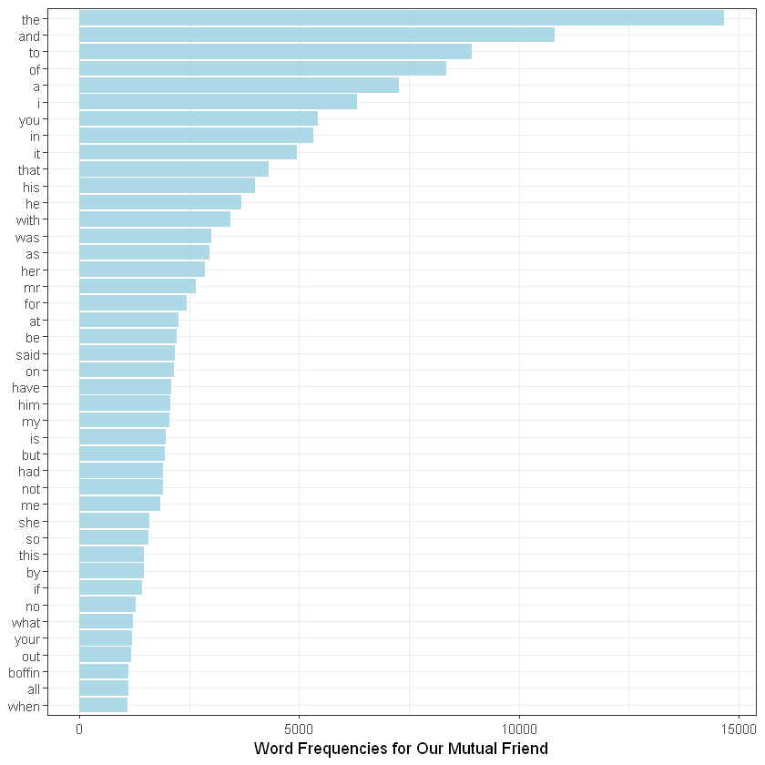
You can change the condition of the filter. I put (n>1000), which means words used more than 1000 times will appear in the analysis. Instead of “lightblue,” you can put other colors. If you type “colors()”, you can find color options. There are 657 colors! In the last line, I put the title.
Notice anything unusual? Most frequent words are stop words, such as “the,” “and,” and “to.” If you want to remove them, you need to remove stopwords from the token_omf file.
data("stop_words")
stop_words
| word | lexicon |
|---|---|
| <chr> | <chr> |
| a | SMART |
| a's | SMART |
| able | SMART |
| about | SMART |
| above | SMART |
| according | SMART |
| accordingly | SMART |
| across | SMART |
| actually | SMART |
| after | SMART |
| afterwards | SMART |
| again | SMART |
| against | SMART |
| ain't | SMART |
| all | SMART |
| allow | SMART |
| allows | SMART |
| almost | SMART |
| alone | SMART |
| along | SMART |
| already | SMART |
| also | SMART |
| although | SMART |
| always | SMART |
| am | SMART |
| among | SMART |
| amongst | SMART |
| an | SMART |
| and | SMART |
| another | SMART |
| ... | ... |
| went | onix |
| were | onix |
| what | onix |
| when | onix |
| where | onix |
| whether | onix |
| which | onix |
| while | onix |
| who | onix |
| whole | onix |
| whose | onix |
| why | onix |
| will | onix |
| with | onix |
| within | onix |
| without | onix |
| work | onix |
| worked | onix |
| working | onix |
| works | onix |
| would | onix |
| year | onix |
| years | onix |
| yet | onix |
| you | onix |
| young | onix |
| younger | onix |
| youngest | onix |
| your | onix |
| yours | onix |
Load stop_words by writing the code above. I will use both the snowball and SMART sets in stop_words, so I did not code to choose either one.
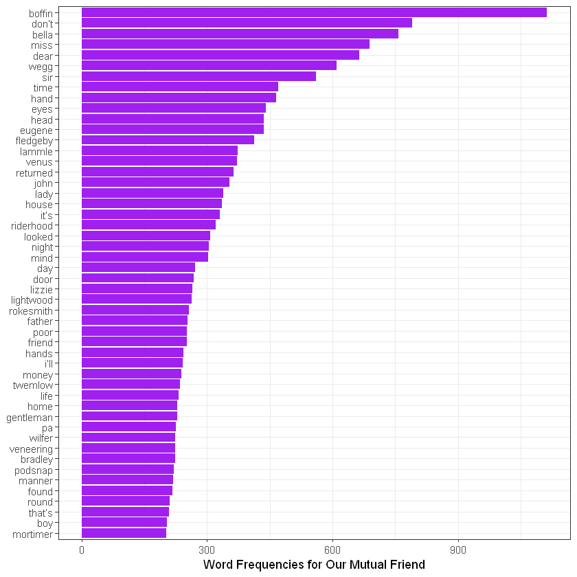
Now, let’s use the anti_join code.
token_omf %>%
count(word, sort = TRUE) %>%
filter(n > 200) %>%
anti_join(stop_words) %>%
mutate(word = reorder(word, n)) %>%
ggplot(aes(word, n)) +
geom_col(fill = "purple") +
xlab(NULL) +
coord_flip() +
theme_bw() +
labs(y = "Word Frequencies for Our Mutual Friend")
Joining, by = "word"
![]()